GasTex | LMF

Last update: February 12, 2024

Remark: Version 3.1 of GasTeX is available here on CTAN since 2024/02/12.

Known problems with TeXLive 2021: If you have problems using gastex simultaneously with the documentclass lipics-v2021, the package todonotes, or the library shadows of tikz (and possibly in other situations), see the known problems and solutions.

For a quick startup guide with some examples, see gastex-doc.tex and the resulting gastex-doc.pdf.

1. Download and Installation

The latest version of GasTeX is always available here. It consists of the following two files:

gastex.sty — contains the definitions of all GasTeX macros.
This file may reside in your working folder but is better placed where other `.sty` files are located, e.g.,

  .../texmf-dist/tex/latex/gastex/gastex.sty

  .../texmf-local/tex/latex/gastex/gastex.sty
  >><<

gastex.pro — contains all the PostScript procedures used to draw the pictures.
This file may also reside in your working folder but is better placed with other `.pro` files, e.g.,

.../texmf-dist/dvips/gastex/gastex.pro

 
.../texmf-local/dvips/gastex/gastex.pro

2. Usage and Package Options

2.1 Usage

\usepackage{gastex}

\usepackage[options]{gastex}

2.2 Package Options

Thanks to the packages pst-pdf and auto-pst-pdf, GasTeX is now fully compatible with pdflatex. This feature is controlled with the two options pdflatex and recompilepics as explained below.

pdflatex — Set this option to true (default) if the LaTeX file is compiled with pdflatex.

\usepackage[pdflatex]{gastex}

\usepackage[pdflatex=true]{gastex}

Omit this option or set it to false if the LaTeX file is compiled with latex+dvips(+ps2pdf).

\usepackage{gastex}

or

\usepackage[pdflatex=false]{gastex}

recompilepics Only with pdflatex — The package pst-pdf includes pictures directly from the file `<jobname>-pics.pdf`. When pictures have changed, this file should be regenerated. This is controlled with the recompilepics option.
\usepackage[pdflatex,recompilepics={false,true,auto}]{gastex} or \usepackage[pdflatex,recompilepics]{gastex}
The possible values for option recompilepics are:
- "auto" (default):
  Computes MD5 checksums of gpicture source code and saves them to `<jobname>-md5.txt`. If checksums differ, you’ll get a warning and the next compilation will regenerate `<jobname>-pics.pdf`.
- "true":
  Forces immediate regeneration of `<jobname>-pics.pdf`, even if unchanged. Useful when modifying pictures repeatedly.
- "false":
  Includes pictures from `<jobname>-pics.pdf` without regenerating, even if sources have changed.

Remarks:

When recompilepics is set to auto or true, the package auto-pst-pdf is loaded and requires compiling with:

pdflatex --shell-escape <jobname>.tex

pdflatex --enable-write18 <jobname>.tex

If not compiling from the command line, you may need to add the shell escape flag in your LaTeX editor’s preferences.

For final submissions to publishers (who often disallow --shell-escape), set recompilepics=false and send `<jobname>-pics.pdf` with your `.tex` source.
To manually generate the PDF for pictures instead of using auto-pst-pdf:

latex <jobname>.tex dvips -o <jobname>-pics.ps <jobname>.dvi ps2pdf <jobname>-pics.ps

auto-pst-pdf options Only with pdflatex — Other options are passed to the package auto-pst-pdf.
- runs=2

\usepackage[pdflatex,recompilepics,runs=2]{gastex}

If a picture uses \ref{}, LaTeX must be run twice to resolve references.

crop=off

\usepackage[pdflatex,recompilepics,crop=off]{gastex}

By default, auto-pst-pdf crops pictures to fit their contents. Set this to "off" to use the dimensions provided in the gpicture environment instead.

3. gpicture and gusepicture

Pictures should be defined inside a gpicture environment, allowing the same source file to be compiled with both pdflatex and latex+dvips(+ps2pdf).

The (deprecated) picture environment may still be used with latex+dvips(+ps2pdf), but it is safe to replace all such environments with gpicture regardless of compilation method.

gpicture

\begin{gpicture}[options]
  ...
\end{gpicture}

\begin{gpicture}[options](width,height)
  ...
\end{gpicture}

\begin{gpicture}[options](width,height)(x offset,y offset)
  ...
\end{gpicture}

The (x offset, y offset) arguments are optional and default to (0,0). The (width, height) arguments are also optional and default to (10,10). All are interpreted in \unitlength. They define a TeX box and its lower-left corner coordinates.

Remark: If compiling with pdflatex and not using the crop=off option, the bounding box is automatically computed and these values are ignored.

The possible options are frame, name, and ignore:

\begin{gpicture}[frame,name=loop,ignore]
  ...
\end{gpicture}

The options name and ignore are only meaningful with pdflatex.

frame={true,false} — default: true.

Adds a visible frame around the picture.

name=<picname>

Gives the picture a name for later reuse with \gusepicture.

ignore={true,false} — default: true. Only with pdflatex

Picture is rendered into `<jobname>-pics.pdf` but not included in the current place. Must be used later via \gusepicture.

gusepicture Only with pdflatex

\gusepicture[options]{<picname>}

Includes picture <picname> which must have been defined with a gpicture environment using the name option.

Useful for reusing pictures or passing extra options to \includegraphics such as clip, viewport, scale, etc.

\gusepicture[viewport=0 5 88 90,clip]{loop}
\gusepicture[viewport=0 5 332 127,scale=0.85]{lessdfs}

Remark: The option clip does not work when added directly to gpicture. This is a known limitation of pst-pdf. Use ignore in gpicture and include the picture later via \gusepicture with the desired clipping options.

4. Drawing Commands

Commands should be used inside the gpicture environment to draw lines, nodes, arrows, etc.

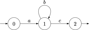
Here is a simple example:

\begin{gpicture}
  \node[Nmarks=i](A)(0,0){0}
  \node(B)(20,0){1}
  \node[Nmarks=f](C)(40,0){2}
  \drawedge(A,B){$a$}
  \drawloop(B){$b$}
  \drawedge(B,C){$c$}
\end{gpicture}

Each drawing command has a name, some optional parameters, and some mandatory arguments:

\commandname[optional parameters]<mandatory arguments>

---

4.1 General Parameters

linegray=<decimal between 0 and 1> — Gray level for drawing edges/lines. `0=black`, `1=white`.
fillgray=<decimal between 0 and 1> — Gray level for filling shapes. `0=black`, `1=white`.
linecolor=<color> — Colour for drawing, e.g., `red`, `blue!40!green`, etc. (uses xcolor).
fillcolor=<color> — Fill colour for nodes or shapes.
linewidth=<number> — Width (in \unitlength) of lines.
dash={pattern}{offset} — Dashed line pattern. `pattern`: list of dash and space lengths. `offset`: where to start the pattern.

 
dash={}{0}
 continuous path  
dash={1.5}{0}
 dashes of length 1.5  
dash={0.2 0.5}{0}
 dotted effect  
dash={4 1 1 1}{0}
 alternating long/short dashes  
dash={1.5}{1.5}
 starts with space  
dash={4}{2}
 starts mid-dash  

4.2 Commands for Nodes (work in progress)

\node — Define and draw a node.

\node(NodeName)(x,y){NodeLabel}
\node[parameter=value,...](NodeName)(x,y){NodeLabel}

- NodeName` is the internal name used in edges, loops, etc. - `(x,y)` are coordinates in \unitlength. - NodeLabel` is any LaTeX content (math, arrays, etc.). Leave empty for no label.

\rpnode — Draw a node shaped as a regular polygon.

\rpnode(NodeName)(x,y)(n,r){NodeLabel}
\rpnode[parameter=value,...](NodeName)(x,y)(n,r){NodeLabel}

- `n` is the number of polygon sides. - `r` is the radius in \unitlength.

\imark — Mark a node as initial with an incoming arrow.

\imark(NodeName)
\imark[parameter=value,...](NodeName)

\fmark — Mark a node as final with an outgoing arrow.

\fmark(NodeName)
\fmark[parameter=value,...](NodeName)

\rmark — Mark a node as repeated (with a second circle).

\rmark(NodeName)
\rmark[parameter=value,...](NodeName)

\nodelabel — Add a label to a node, possibly multiple times at various angles.

\nodelabel(NodeName){NodeLabel}
\nodelabel[parameter=value,...](NodeName){NodeLabel}

---

Examples: Nodes and Labels

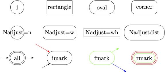
\begin{gpicture}
  \gasset{Nw=8,Nh=8}
  \node(A)(0,0){1}
  \node[Nw=15,Nmr=0](A)(25,0){rectangle}
  \node[Nw=15,Nmr=4](A)(50,0){oval}
  \node[Nw=15,Nmr=2](A)(75,0){corner}

  \node(B)(0,-15){Nadjust=n}
  \node[Nadjust=w,Nmr=2](B)(25,-15){Nadjust=w}
  \node[Nadjust=wh,Nmr=0](B)(50,-15){Nadjust=wh}
  \node[Nadjust=wh,Nadjustdist=3](B)(75,-15){Nadjustdist}

  \gasset{Nadjust=w,Nadjustdist=3}
  \node[Nmarks=ifr](C)(0,-30){all}
  \node[Nmarks=i,iangle=210,ilength=5](C)(25,-30){imark}
  \imark[iangle=150,ilength=10,linecolor=red](C)
  \node[Nmarks=f,fangle=30,flength=5,linecolor=green](C)(50,-30){fmark}
  \fmark[fangle=-30,flength=10,linecolor=blue](C)
  \node[Nmarks=r,linecolor=red](C)(75,-30){rmark}
  \rmark[rdist=1.4,linecolor=green](C)
\end{gpicture}

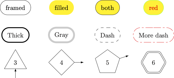
\begin{gpicture}
  \gasset{Nadjust=w,Nadjustdist=3,Nh=8}
  \node(D)(0,0){framed}
  \node[Nframe=n,fillcolor=yellow](D)(25,0){filled}
  \node[fillcolor=yellow](D)(50,0){both}
  \node[fillcolor=yellow,linecolor=green](D)(75,0){\textcolor{red}{red}}

  \node[linewidth=0.5](E)(0,-15){Thick}
  \node[linewidth=1,linegray=0.8](E)(25,-15){Gray}
  \node[dash={1.5}0](E)(50,-15){Dash}
  \node[dash={4 1 1 1}0,linecolor=red](E)(75,-15){More dash}

  \rpnode[polyangle=90,Nmarks=i,iangle=-90](F)(0,-30)(3,7){3}
  \rpnode[Nmarks=f](F)(25,-30)(4,7){4}
  \rpnode[polyangle=90,Nmarks=f,fangle=18](F)(50,-30)(5,7){5}
  \rpnode[arcradius=2,Nmarks=r](F)(75,-30)(6,7){6}
\end{gpicture}

\begin{gpicture}
  {\gasset{Nfill=y,Nw=2,Nh=2,ExtNL=y,NLdist=1.5}
  \node(A)(0,0){$a$}
  \node[NLangle=-90](B)(10,0){$b$}
  \drawedge(A,B){}
  \drawloop[loopdiam=5](B){}
  }

  \gasset{ExtNL=n,NLdist=10}
  \node[Nh=24,Nw=24,Nmr=12](B)(40,0){}
  \nodelabel[NLangle=  0](B){3}
  \nodelabel[NLangle= 30](B){2}
  \nodelabel[NLangle= 60](B){1}
  \nodelabel[NLangle= 90](B){12}
  \nodelabel[NLangle=120](B){11}
  \nodelabel[NLangle=150](B){10}
  \nodelabel[NLangle=180](B){9}
  \nodelabel[NLangle=210](B){8}
  \nodelabel[NLangle=240](B){7}
  \nodelabel[NLangle=270](B){6}
  \nodelabel[NLangle=300](B){5}
  \nodelabel[NLangle=330](B){4}

  \node[Nh=20,Nw=20,Nmr=10](D)(75,0){}
  \gasset{ExtNL=y,NLdist=1,AHnb=0,ilength=-2}
  \nodelabel[NLangle=  0](D){3}  \imark[iangle=  0](D)
  \nodelabel[NLangle= 30](D){2}  \imark[iangle= 30](D)
  \nodelabel[NLangle= 60](D){1}  \imark[iangle= 60](D)
  \nodelabel[NLangle= 90](D){12} \imark[iangle= 90](D)
  \nodelabel[NLangle=120](D){11} \imark[iangle=120](D)
  \nodelabel[NLangle=150](D){10} \imark[iangle=150](D)
  \nodelabel[NLangle=180](D){9}  \imark[iangle=180](D)
  \nodelabel[NLangle=210](D){8}  \imark[iangle=210](D)
  \nodelabel[NLangle=240](D){7}  \imark[iangle=240](D)
  \nodelabel[NLangle=270](D){6}  \imark[iangle=270](D)
  \nodelabel[NLangle=300](D){5}  \imark[iangle=300](D)
  \nodelabel[NLangle=330](D){4}  \imark[iangle=330](D)
\end{gpicture}

4.3 Commands for Edges (work in progress)

\drawedge — Draw a straight edge between two nodes.

\drawedge(startNode,endNode){EdgeLabel}
\drawedge[parameter=value,...](startNode,endNode){EdgeLabel}

- `startNode`, `endNode`: names of previously defined nodes. - EdgeLabel`: any LaTeX content. Leave empty if no label.

\drawloop — Draw a loop on a node using a cubic Bézier curve.

\drawloop(NodeName){EdgeLabel}
\drawloop[parameter=value,...](NodeName){EdgeLabel}

- NodeName`: a defined node name. - EdgeLabel`: optional label.

\drawqbedge — Draw a quadratic Bézier edge between two nodes using a control point.

\drawqbedge(start,x,y,end){EdgeLabel}
\drawqbedge[parameter=value,...](start,x,y,end){EdgeLabel}

- `(x,y)`: coordinates of the control point in \unitlength.

\drawqbpedge — Same as above, but with polar angles at endpoints instead of coordinates.

\drawqbpedge(start,sa,end,ea){EdgeLabel}
\drawqbpedge[parameter=value,...](start,sa,end,ea){EdgeLabel}

- `sa`, `ea`: angles (in degrees) for source/target Bézier control points.

\drawcbedge — Cubic Bézier edge with two intermediate control points.

\drawcbedge(start,xs,ys,end,xe,ye){EdgeLabel}
\drawcbedge[parameter=value,...](start,xs,ys,end,xe,ye){EdgeLabel}

- `(xs,ys)` and `(xe,ye)` are the two control points.

\drawcbpedge — Cubic Bézier edge with polar coordinates for control points.

\drawcbpedge(start,sa,sr,end,ea,er){EdgeLabel}
\drawcbpedge[parameter=value,...](start,sa,sr,end,ea,er){EdgeLabel}

- `sa`, `sr`: angle and radius from start node. - `ea`, `er`: angle and radius from end node.

Examples for `\drawedge, \drawloop, \drawqbedge, \drawqbpedge, \drawcbedge, \drawcbpedge`

\begin{gpicture}
  \gasset{Nadjust=wh,Nadjustdist=2,loopdiam=6}
  \node[Nmarks=i,iangle=200,fillcolor=yellow](A)(-20,0){initial}
  \node[Nmarks=f,Nmr=0,fillgray=0.85,dash={1}0](B)(20,0){final}
  \node[Nmarks=r,Nmr=3,linecolor=green](C)(60,0){$\left( \begin{array}{ccc} 2 & 1 & 0 \\ -1 & 0 & 1 \\ 0 & -1 & 2 \end{array}\right)$}
  \rmark[linecolor=green,rdist=1.4](C)

  \drawedge[ELside=r,ELpos=35](A,B){straight}
  \drawedge[curvedepth=5,linecolor=red](A,B){\textcolor{blue!50!white}{curved}}
  \drawedge[curvedepth=-15,ELdist=2,dash={1.5}0](A,B){far}

  \drawloop[ELpos=75,ELdist=-1,loopangle=150,dash={0.2 0.5}0](A){clockwise}
  \drawloop[ELpos=70,loopangle=-90,loopwidth=3](A){$b\mid 10$}
  \drawloop[loopCW=n,ELside=r](B){counter-CW}

  \drawqbpedge[ELside=r,dash={4 1 1 1}0](B,-90,C,210){qbpedge}
  \drawloop[ELside=r,loopangle=-90,loopwidth=5](C){$a$}
\end{gpicture}

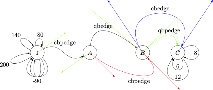
\begin{gpicture}
  \node(1)(10,0){1}
  \gasset{loopangle=-90,loopheight=10}
  \drawloop {}
  \drawloop {}
  \drawloop {-90}
  \gasset{loopwidth=4}
  \drawloop {80}
  \drawloop {140}
  \drawloop {200}

  \node(A)(40,0){$A$}
  \drawcbpedge[ELpos=40,ELdist=0](1,35,20,A,-145,20){cbpedge}
  \drawline[linecolor=green](10,0)(26.4,11.5)
  \drawline[linecolor=green](40,0)(23.6,-11.5)

  \node(B)(70,0){$B$}
  \drawqbedge(A,40,25,B){qbedge}
  \drawline[linecolor=green,AHnb=0](40,0)(40,25)(70,0)

  \drawcbpedge[linecolor=red,ELside=r](A,-45,20,B,-45,30){cbpedge}
  \drawline[linecolor=red](40,0)(54.14,-14.14)
  \drawline[linecolor=red](70,0)(91.21,-21.21)

  \node(C)(90,0){$C$}
  \drawcbedge[linecolor=blue](B,50,30,C,110,30){cbedge}
  \drawline[linecolor=blue](70,0)(50,30)
  \drawline[linecolor=blue](90,0)(110,30)

  \drawqbpedge[linecolor=green](B,45,C,90){qbpedge}
  \drawline[linecolor=green,AHnb=0](70,0)(90,20)(90,0)

  \gasset{ELside=r}
  \drawloop[loopdiam=12](C){12}
  \drawloop[loopdiam=8,loopangle=0](C){8}
  \drawloop[loopdiam=6,loopangle=-90](C){6}
\end{gpicture}

4.4 Lines and Curves

\drawline — Draw a broken line defined by n points (n > 1).

\drawline(x1,y1)...(xn,yn)
\drawline[parameter=value,...](x1,y1)...(xn,yn)

- Each pair `(x, y)` gives the coordinates in \unitlength. - The result may include arrowheads, colours, dash patterns, etc.

\drawcurve — Draw a smooth continuous curve through n points (n > 1).

\drawcurve(x1,y1)...(xn,yn)
\drawcurve[parameter=value,...](x1,y1)...(xn,yn)

- Between each pair of points, a cubic Bézier curve is drawn. - Control points are computed to ensure smoothness and orthogonality to the angle bisectors. - Optional parameters as for \drawline.

Examples for `\drawline` and `\drawcurve`

\begin{gpicture}
  \gasset{AHnb=0}
  \put(2,3){\unitlength=8mm
    \drawline(0,0)(0,2)(1,3)(0,4)(2,4)(2,2)(4,0)(2,0)(1,1)
    \drawcurve[linecolor=red](0,0)(0,2)(1,3)(0,4)(2,4)(2,2)(4,0)(2,0)(1,1)
  }

  \put(7,5){\unitlength=8mm
    \drawline[linecolor=blue,arcradius=.2](0,0)(0,2)(1,3)(0,4)(2,4)(2,2)(4,0)(2,0)(1,1)
  }

  \put(55,16){\unitlength=1.5mm
    \drawline(-10,-10)(10,10)(-10,10)(10,-10)
    \drawcurve[linecolor=red,ATnb=3,AHnb=4](-10,-10)(10,10)(-10,10)(10,-10)
  }

  \put(100,19){\unitlength=20mm
    \drawline(0.95,0.3)(-0.59,-0.8)(0,1)(0.59,-0.8)(-0.95,0.3)
    \drawcurve[linecolor=red,AHnb=1](0.95,0.3)(-0.59,-0.8)(0,1)(0.59,-0.8)(-0.95,0.3)
  }
\end{gpicture}

4.5 Polygons and Closed Curves

\drawpolygon — Draw a polygon defined by a sequence of at least two points.

\drawpolygon(x1,y1)...(xn,yn)
\drawpolygon[parameter=value,...](x1,y1)...(xn,yn)

- Coordinates are interpreted in \unitlength. - Optional parameters allow for framing, filling, dashing, etc.

\drawccurve — Draw a smooth closed curve through a sequence of points.

\drawccurve(x1,y1)...(xn,yn)
\drawccurve[parameter=value,...](x1,y1)...(xn,yn)

- Uses cubic Bézier curves to connect the points smoothly. - Optional parameters as above.

Examples for `\drawpolygon` and `\drawccurve`

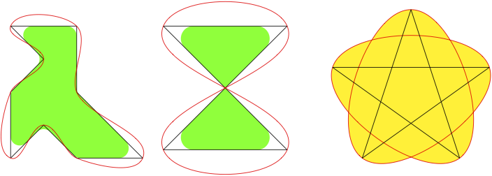
\begin{gpicture}
  \put(3,3){\unitlength=8mm
    \drawpolygon[fillcolor=green,Nframe=n,arcradius=.3](0,0)(0,2)(1,3)(0,4)(2,4)(2,2)(4,0)(2,0)(1,1)
    \drawpolygon(0,0)(0,2)(1,3)(0,4)(2,4)(2,2)(4,0)(2,0)(1,1)
    \drawccurve[linecolor=red](0,0)(0,2)(1,3)(0,4)(2,4)(2,2)(4,0)(2,0)(1,1)
  }

  \put(55,20){\unitlength=1.5mm
    \drawpolygon[fillcolor=green,Nframe=n,arcradius=2](-10,-10)(10,10)(-10,10)(10,-10)
    \drawpolygon(-10,-10)(10,10)(-10,10)(10,-10)
    \drawccurve[linecolor=red](-10,-10)(10,10)(-10,10)(10,-10)
  }

  \put(100,19){\unitlength=20mm
    \drawccurve[fillcolor=yellow,linecolor=red](0,1)(0.59,-0.8)(-0.95,0.3)(0.95,0.3)(-0.59,-0.8)
    \drawpolygon(0,1)(0.59,-0.8)(-0.95,0.3)(0.95,0.3)(-0.59,-0.8)
  }
\end{gpicture}

4.6 Circles and Arcs

\drawcircle — Draw a circle.

\drawcircle(x,y,d)
\drawcircle[parameter=value,...](x,y,d)

- `(x, y)`: coordinates of the centre - `d`: diameter (all in \unitlength) - Can be framed or filled with optional parameters.

\drawarc — Draw an arc of a circle.

\drawarc(x,y,r,a,b)
\drawarc[parameter=value,...](x,y,r,a,b)

- `(x, y)`: coordinates of the centre - `r`: radius - `a`, `b`: start and end angles in degrees - Can be framed and/or filled - Use arcPie=y to fill the area between the arc and the centre

Examples for `\drawcircle` and `\drawarc`

\begin{gpicture}[name=circles-arcs]
  \drawcircle[Nfill=y,fillcolor=blue](0,0,40)
  \drawcircle[Nfill=y,fillcolor=white](0,0,30)
  \drawcircle[Nfill=y,fillcolor=red](0,0,20)
  \drawcircle[Nfill=y,fillcolor=yellow](0,0,10)

  \drawarc[linecolor=black](50,0,20,0,45)
  \drawarc[arcPie=y,linecolor=blue](50,0,20,-50,-15)
  \drawarc[fillcolor=red,linecolor=red](50,0,20,90,190)
  \drawarc[arcPie=y,fillcolor=yellow,linecolor=yellow](50,0,20,200,250)
  \drawarc[arcPie=y,linecolor=blue](100,0,20,-15,-50)
\end{gpicture}

4.7 Rectangles, Ovals and Regular Polygons

\drawrect — Draw a rectangle.

\drawrect(x0,y0,x1,y1)
\drawrect[parameter=value,...](x0,y0,x1,y1)

- `(x0,y0)` and `(x1,y1)` are the coordinates (in \unitlength) of the lower-left and upper-right corners. - Optional parameters allow framing, filling, etc.

\drawoval — Draw an oval (a rectangle with rounded corners).

\drawoval(x,y,w,h,mr)
\drawoval[parameter=value,...](x,y,w,h,mr)

- `(x,y)` is the centre - `w` and `h` are width and height - `mr` is the maximum radius of rounded corners (0 = normal rectangle)

\drawrpolygon — Draw a regular polygon.

\drawrpolygon(x,y)(n,r)
\drawrpolygon[parameter=value,...](x,y)(n,r)

- `(x,y)` is the centre - `n` is the number of sides - `r` is the radius of the circumscribed circle - Optional parameters allow filling, rotation (`polyangle`), etc.

Examples for `\drawrect`, `\drawoval` and `\drawrpolygon`

\begin{gpicture}
  \drawrpolygon[polyangle=90,fillcolor=blue](0,0)(3,8)
  \drawrpolygon[fillcolor=green](20,0)(4,7)
  \drawrpolygon[polyangle=18,arcradius=5](40,0)(5,7)
  \drawrpolygon(60,0)(8,7)
  \drawrpolygon(60,0)(8,6)
  \drawrpolygon(60,0)(8,5)

  \drawrect[Nfill=y,fillcolor=yellow](75,-5,95,5)
  \drawrect[arcradius=3,dash={1.2}0](77,-4,93,4)

  \drawoval(115,0,20,10,3)
  \drawoval[Nfill=y,fillcolor=green](115,0,15,8,5)
  \drawoval[Nfill=y,fillcolor=red](115,0,10,4,0)
\end{gpicture}

4.8 Bézier Curves and Snake Lines

\drawqbezier — Draw a quadratic Bézier curve.

\drawqbezier(x0,y0,x1,y1,x2,y2)
\drawqbezier[parameter=value,...](x0,y0,x1,y1,x2,y2)

- `(x0,y0)` is the start point - `(x1,y1)` is the control point - `(x2,y2)` is the end point - Units in \unitlength

\drawcbezier — Draw a cubic Bézier curve.

\drawcbezier(x0,y0,x1,y1,x2,y2,x3,y3)
\drawcbezier[parameter=value,...](x0,y0,x1,y1,x2,y2,x3,y3)

- `(x0,y0)`: start - `(x1,y1)` and `(x2,y2)`: control points - `(x3,y3)`: end point

\drawsnake — Draw a snake-style wavy line.

\drawsnake(x1,y1)(x2,y2)
\drawsnake[parameter=value,...](x1,y1)(x2,y2)

- `(x1,y1)` to `(x2,y2)` defines the start and end of the wave - Parameters such as snakeh and snakew control height and wavelength

Examples for `\drawqbezier, \drawcbezier, \drawsnake`

\begin{gpicture}
  \gasset{AHnb=0}
  \drawline[linecolor=green](0,0)(-5,15)(20,0)
  \drawqbezier(0,0,-5,15,20,0)

  \drawline[linecolor=green](0,-2)(10,-12)(20,-2)
  \drawqbezier[linecolor=blue,AHnb=2](0,-2,10,-12,20,-2)

  \gasset{AHnb=1}
  \drawline[linecolor=green](25,0)(15,10)
  \drawline[linecolor=green](25,0)(35,10)
  \drawcbezier[linecolor=red](25,0,15,10,35,10,25,0)

  \drawline[linecolor=green](30,0)(40,0)
  \drawline[linecolor=green](50,15)(40,15)
  \drawcbezier[AHnb=0,dash={1.5}0](30,0,40,0,40,15,50,15)

  \drawline[linecolor=green](70,10)(90,0)
  \drawline[linecolor=green](70,-10)(50,0)
  \drawcbezier[linecolor=blue](70,10,90,0,50,0,70,-10)

  \drawsnake[linecolor=red,snakeh=.8,snakew=.8](100,10)(120,10)
  \drawsnake[linecolor=blue,snakeh=2,snakew=1](100,0)(120,0)
  \drawsnake[linecolor=green,snakeh=3.5,snakew=1.9](100,-10)(120,-10)
\end{gpicture}

5. More Examples

The documentation above already contains many examples. Some additional examples are available in the following files:

gastex-examples.tex and gastex-examples.pdf — Learn gastex and test your installation.
gastex-gusepicture.tex and gastex-gusepicture.pdf — How to compile gastex pictures with pdflatex.

6. Known problems and (hopefully) solutions

Documentclass lipics-v2021 and TeXLive 2021 (2021/10/21): Starting with version 2021 of the documentclass lipics, an error appears when compiling gastex pictures with pdflatex=true. The error occurs during the latex+dvips+ps2pdf step, likely due to recent versions of hyperref and/or preview. Solution: Remove the hooks set by hyperref when the compilation is not in pdf mode:

\documentclass[a4paper,UKenglish]{lipics-v2021}
\usepackage[pdflatex,recompilepics=true]{gastex}
\ifpdf
  \usepackage{todonotes}
  \RequirePackage{tikz}
  \usetikzlibrary{shadows}
\else
  \AtBeginDocument{%
    \RemoveFromHook{shipout/firstpage}[hyperref]%
    \RemoveFromHook{shipout/before}[hyperref]%
  }
\fi
\begin{document}
...

Package todonotes or TikZ shadows library (2021/10/21): An error also appears when using todonotes or the shadows TikZ library under pdflatex=true with TeXLive 2021. Solution: Load these packages only if the compilation is in pdf mode:

\documentclass{article}
\usepackage[pdflatex,recompilepics=true]{gastex}
\ifpdf
  \usepackage{todonotes}
  \RequirePackage{tikz}
  \usetikzlibrary{shadows}
\fi
\begin{document}
...

Overlays with Beamer and pdflatex (2012/08/21): When a Beamer frame consists only of a gpicture, only the first overlay may be shown under pdflatex. Likely a problem with auto-pst-pdf or beamer. Solution: Add a command outside the gpicture to trigger overlay generation, e.g., \pause[6].
gasset inside tabular or array (2000/10/27): Using gasset inside tabular or array may cause an error because & is used as an internal marker. Solution: Wrap the picture in an \mbox{}.

\begin{tabular}{c}
  \mbox{
    \begin{picture}(10,20)(-5,-5)
      \gasset{ELdist=0}
      \node(A)(0,0){1}
      \drawloop(A){$a$}
    \end{picture}
  }
\end{tabular}

GasTeX and German package (1999/10/21): When using gastex with the german package (loaded first), dvips may fail. Solution: Load gastex before german.

\usepackage{gastex}
\usepackage{german}

I do not know the root cause of this issue.

7. Feedback

I hope you will find GasTeX helpful. Let me know if you have any problem or suggestion to improve it.

Paul Gastin GasTeX: Graphs and Automata Simplified in TeX

version 3.1

1. Download and Installation

2. Usage and Package Options

2.1 Usage

2.2 Package Options

3. gpicture and gusepicture

4. Drawing Commands

4.1 General Parameters

4.2 Commands for Nodes (work in progress)

Examples: Nodes and Labels

4.3 Commands for Edges (work in progress)

Examples for `\drawedge, \drawloop, \drawqbedge, \drawqbpedge, \drawcbedge, \drawcbpedge`

4.4 Lines and Curves

Examples for `\drawline` and `\drawcurve`

4.5 Polygons and Closed Curves

Examples for `\drawpolygon` and `\drawccurve`

4.6 Circles and Arcs

Examples for `\drawcircle` and `\drawarc`

4.7 Rectangles, Ovals and Regular Polygons

Examples for `\drawrect`, `\drawoval` and `\drawrpolygon`

4.8 Bézier Curves and Snake Lines

Examples for `\drawqbezier, \drawcbezier, \drawsnake`

5. More Examples

6. Known problems and (hopefully) solutions

7. Feedback

Contact

`dash={}{0}`	continuous path
`dash={1.5}{0}`	dashes of length 1.5
`dash={0.2 0.5}{0}`	dotted effect
`dash={4 1 1 1}{0}`	alternating long/short dashes
`dash={1.5}{1.5}`	starts with space
`dash={4}{2}`	starts mid-dash

Paul Gastin GasTeX: Graphs and Automata Simplified in TeX

version 3.1

1. Download and Installation

2. Usage and Package Options

2.1 Usage

2.2 Package Options

3. gpicture and gusepicture

4. Drawing Commands

4.1 General Parameters

4.2 Commands for Nodes (work in progress)

Examples: Nodes and Labels

4.3 Commands for Edges (work in progress)

Examples for \drawedge, \drawloop, \drawqbedge, \drawqbpedge, \drawcbedge, \drawcbpedge

4.4 Lines and Curves

Examples for \drawline and \drawcurve

4.5 Polygons and Closed Curves

Examples for \drawpolygon and \drawccurve

4.6 Circles and Arcs

Examples for \drawcircle and \drawarc

4.7 Rectangles, Ovals and Regular Polygons

Examples for \drawrect, \drawoval and \drawrpolygon

4.8 Bézier Curves and Snake Lines

Examples for \drawqbezier, \drawcbezier, \drawsnake

5. More Examples

6. Known problems and (hopefully) solutions

7. Feedback

Contact

Examples for `\drawedge, \drawloop, \drawqbedge, \drawqbpedge, \drawcbedge, \drawcbpedge`

Examples for `\drawline` and `\drawcurve`

Examples for `\drawpolygon` and `\drawccurve`

Examples for `\drawcircle` and `\drawarc`

Examples for `\drawrect`, `\drawoval` and `\drawrpolygon`

Examples for `\drawqbezier, \drawcbezier, \drawsnake`